
 The All-Reduce collective is ubiquitous in distributed training, but is currently not supported for sparse CUDA tensors in PyTorch. In the first part of this blog we contrast the existing alternatives available in the Gloo/NCCL backends. In the second part we implement our own efficient sparse All-Reduce collective using PyTorch and CUDA.
Sparse embeddings, what are they good for?
The torch.nn.Embedding layer in PyTorch provides a sparse option to store the embedding weights as a sparse (COO) tensor. This allows us to improve performance and reduce memory footprint, by only computing/storing the gradients of parameters which contributed to the forward pass.
The example below shows an embedding gradient tensor when using the default sparse=False. This approach stores gradients for all embeddings, even though only two embeddings have been utilized in the forward pass.
import torch

x = torch.tensor([1, 3])

embedding = torch.nn.Embedding(8, 4, sparse=False)
embedding(x).sum().backward()

print(embedding.weight.grad)
tensor([[0., 0., 0., 0.],
        [1., 1., 1., 1.],
        [0., 0., 0., 0.],
        [1., 1., 1., 1.],
        [0., 0., 0., 0.],
        [0., 0., 0., 0.],
        [0., 0., 0., 0.],
        [0., 0., 0., 0.]])
In comparison, the sparse variant only stores the values of the non-zero gradients and the indices that reference them.
sparse_embedding = torch.nn.Embedding(8, 4, sparse=True)
sparse_embedding(x).sum().backward()

print(sparse_embedding.weight.grad)
tensor(indices=tensor([[1, 3]]),
       values=tensor([[1., 1., 1., 1.],
                      [1., 1., 1., 1.]]),
       size=(8, 4), nnz=2, layout=torch.sparse_coo)
The efficiency of sparse=True is particularly appealing when dealing with very large embeddings, where only a small fraction of the elements contribute to a single parameter update. This can be common in language modelling tasks which sample tokens from a large vocabulary into a single mini-batch, or when a contrastive objective function requires drawing a small number of negative samples (e.g. NCE).
Sparse All-Reduce
A further benefit of sparse gradients can be found in the distributed setting. With less data to communicate between GPUs via All-Reduce in the backward pass, we can see further performance gains. Unfortunately, a sparse version of All-Reduce is not available for the NCCL distributed backend. PyTorch currently only supports sparse All-Reduce with the Gloo backend, which means by-passing the blazingly fast NVLinks and falling back to PCIe 🥲
When running torch.distributed.all_reduce on a CUDA based sparse tensor this is the result
RuntimeError: Tensors must be CUDA and dense
Our ultimate goal here is to implement a sparse All-Reduce which utilizes the NCCL collectives and keeps the GPUs cooking 🔥
Before jumping into the implementation, we will fist look at the performance of existing options currently available in PyTorch.
Measuring the embedding layer performance for dense All-Reduce is trivial, and scales with the total number of embeddings in the full tensor. However when measuring the relative uplift of sparse All-Reduce we also need to consider the sparsity level. That is, the percentage of elements from the full dense tensor which are zero and do not need to be communicated.
We initially consider two simple baselines to benchmark, using the Gloo and NCCL backends
def all_reduce_gloo(x):
    x = x.coalesce().cpu()
    torch.distributed.all_reduce(x)
    return x.cuda()
For the Gloo baseline we ensure that the data originates in GPU memory and is copied to CPU (and back again after reduction). As we are trying to synchronize GPU based gradients, the cost of moving the data onto the host for the all_reduce must be factored in1.
Note that we coalesce() prior to copying to CPU. This is important because the sparse tensor produced by autograd will be uncoalesced. This means that any embedding that has been sampled more than once will have duplicate value entries stored. By coalescing we sum the entries that share the same index. This happens implicitly in the all_reduce call, but by calling it prior to the copy we reduce the amount of data we need to transfer to the host, which improves performance. Here's an example:
indices = torch.tensor([[2, 2, 3]])
values = torch.randn(3, 4)

x = torch.sparse_coo_tensor(indices, values, size=(5,4))
print(x)
tensor(indices=tensor([[2, 2, 3]]),
       values=tensor([[ 0.4746, -0.0639,  0.0267, -0.9349],
                      [ 1.7140, -1.8417, -1.0404,  0.7796],
                      [ 1.5173,  1.0823, -1.3910,  1.0001]]),
       size=(5, 4), nnz=3, layout=torch.sparse_coo)
print(x.coalesce())
tensor(indices=tensor([[2, 3]]),
       values=tensor([[ 2.1886, -1.9056, -1.0137, -0.1552],
                      [ 1.5173,  1.0823, -1.3910,  1.0001]]),
       size=(5, 4), nnz=2, layout=torch.sparse_coo)
The second baseline simply materializes the sparse tensor into its dense counterpart prior to communication, in order to utilize the NCCL backend.
def all_reduce_nccl_dense(x):
    x_dense = x.to_dense()
    torch.distributed.all_reduce(x_dense)
    indices = x_dense.abs().max(dim=1)[0].nonzero().squeeze(1)
    values = x_dense[indices]
    return torch.sparse_coo_tensor(indices.unsqueeze(0), values, size=x_dense.shape, device=device)
Note that we build a new set of indices for the reduced output tensor, rather than using x.indices(). This is because the number of non-zero local embeddings will be ≤ the total number of non-zero embeddings contributing to the collective across all ranks, as each rank will sample different embeddings (e.g. each local mini-batch will contain different tokens).
Baseline results
For our initial experiments we consider a total embedding size of 5e6, a feature dim of 2048 and a sparsity level of ~99% (giving ~50,000 embeddings sampled on each local rank). Tests are carried out across 8 GPUs in a DGX H100 SXM node, and utilizing the NVSwitch for NCCL based collectives.

We can clearly see that throughput for the naive dense+NCCL baseline is an order of magnitude higher than sparse+Gloo, despite the fact that we are transporting more data. There could be a number of reasons for this:
- NCCL vs. Gloo: Differences in NCCL/Gloo protocol overhead, and implementation details of the collective algorithm (e.g. ring vs. tree-based All-Reduce)
- Dense vs. Sparse: The sparse All-Reduce transmits less data overall, but there may be other costs not present in the dense equivalent. We look closer at this in Part 2.
- NVLink vs. PCIe: Lack of NVSwitch availability in Gloo setup resulting in lower communication bandwidth.
NVLink vs. PCIe
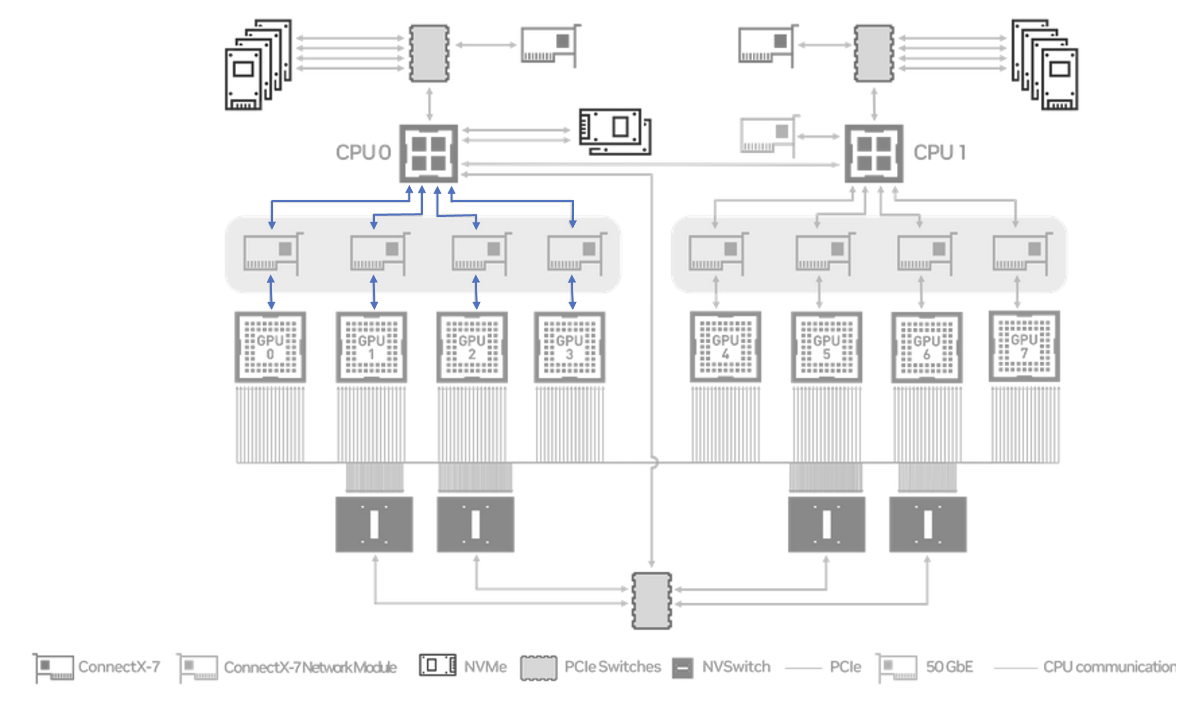
The last point is particularly important. NCCL can exploit the high interconnect bandwidth provided by the NVLinks, and their attached NVSwitches. Without this we would have to fall back to transmitting data via the PCIe links, and across the UPI interconnect between the CPUs. To illustrate this difference the diagram below has the NVLink (NCCL) based transport path highlighted in green, and the PCIe/UPI (Gloo) path highlighted in blue/red.
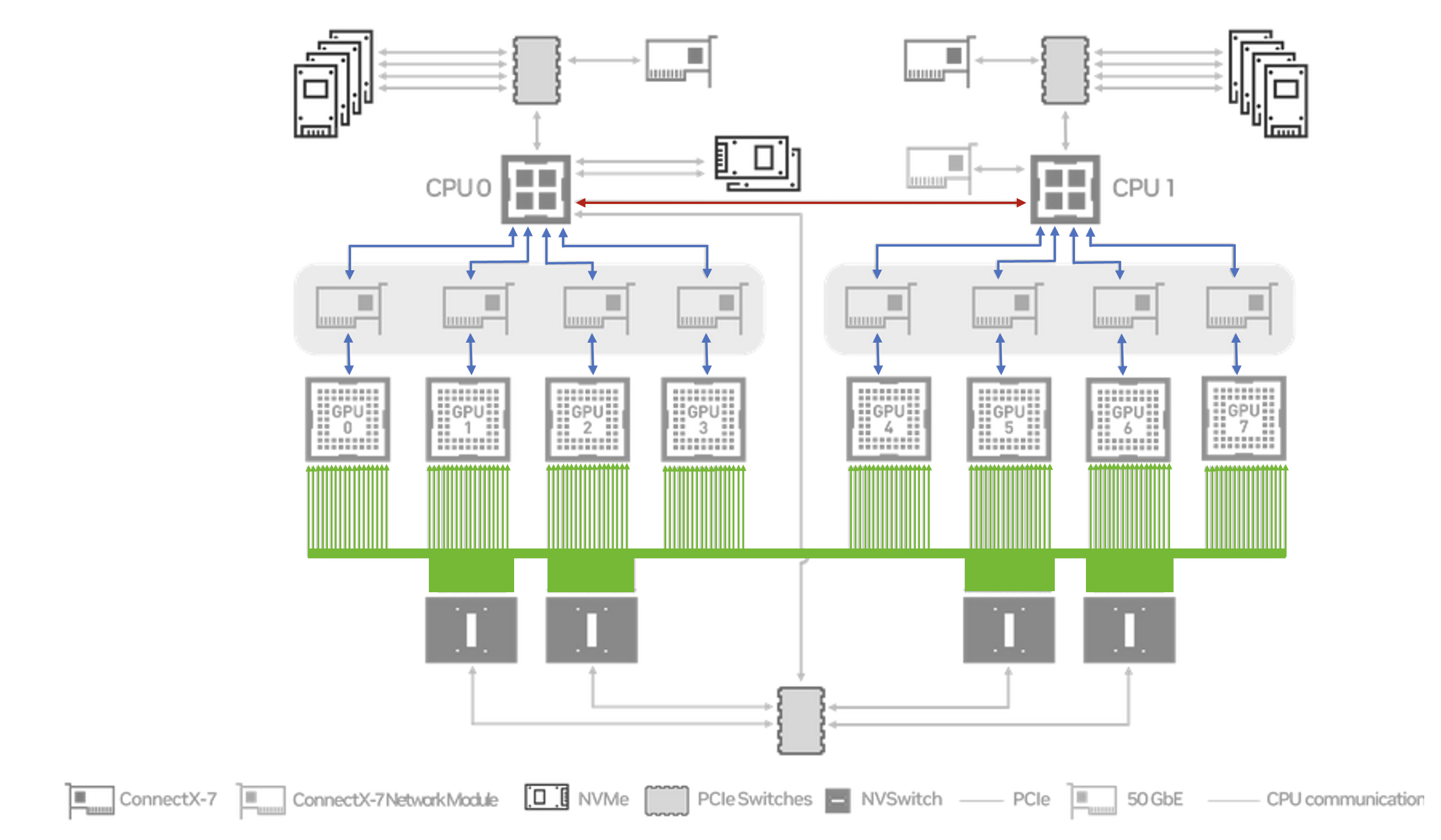
Each H100 GPU has 18 NVLinks attached to it, providing a total of 450 GB/s of intra-node communication bandwidth to each card (in each direction). In contrast the PCIe 5.0 links only support up to 63 GB/s unidirectional bandwidth, and a total of 64 GB/s across the UPI links between the CPUs.
Despite the 450 GB/s line rate provided by the NVLinks, in practise we measure ~362 GB/s of peak bandwidth, due to the ~20% overhead incurred by the NCCL protocol. This test is carried out using the all_reduce_perf executable in nccl-tests.
#       size         count      type   redop    root     time   bandwidth
  1073741824     268435456     float     sum      -1   5187.6      362.22
Whilst we cannot disable NVLink directly in order to get comparative numbers using the PCIe path, we can disable peer-to-peer communication with NCCL_P2P_DISABLE=1. This has the effect of forcing NCCL onto a path that does not require P2P i.e. PCIe via CPU. We can confirm NCCL_P2P_DISABLE=1 is not using NVLink by checking no data is transmitted over NVLink with nvidia-smi nvlink -gt d.
After setting NCCL_P2P_DISABLE=1 and running the all_reduce_perf benchmark our peak bandwidth is now only ~24 GB/s.
#       size         count      type   redop    root     time   bandwidth
  1073741824     268435456     float     sum      -1    78895       23.82
This clearly illustrates the performance gains we get from utilizing the NVLink, although there is a caveat. Disabling P2P is only a proxy for what we want to test: "Does lack of NVLink account for the gap we saw between sparse+Gloo and dense+NCCL?" . Our approach disables all P2P data movement, including P2P over PCIe. Without P2P we have to fall-back to using an intermediate read/write to shared memory.
This means we are effectively seeing a lower bound for performance without NVLink. We measure a ~15x reduction in throughput when the theoretical drop-off (450/64) is closer to 7x. Is PCIe without P2P a good approximation for PCIe with P2P performance? We can get some insight here by considering the PCIe based communication patterns.
Impact of P2P
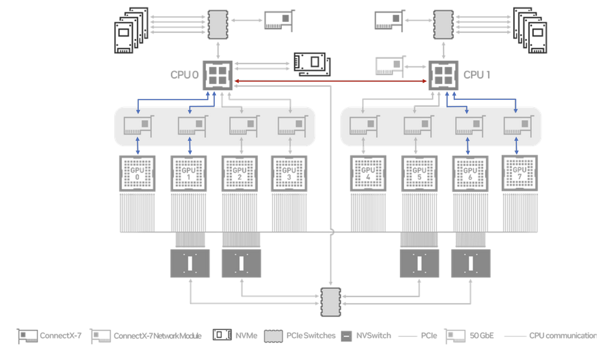
Unlike the homogeneous NVLink path (where a subset of each GPU's NVLinks are connected to every NVSwitch), the PCIe path in the DGX has two distinct patterns: communication between GPUs within the same NUMA node (GPUs connected to the same CPU) and communication across NUMA nodes (which uses the UPI connection). The topology provided by nvidia-smi topo -mp illustrates this.
        GPU0    GPU1    GPU2    GPU3    GPU4    GPU5    GPU6    GPU7   NUMA
GPU0     X      NODE    NODE    NODE    SYS     SYS     SYS     SYS      0
GPU1    NODE     X      NODE    NODE    SYS     SYS     SYS     SYS      0
GPU2    NODE    NODE     X      NODE    SYS     SYS     SYS     SYS      0
GPU3    NODE    NODE    NODE     X      SYS     SYS     SYS     SYS      0
GPU4    SYS     SYS     SYS     SYS      X      NODE    NODE    NODE     1
GPU5    SYS     SYS     SYS     SYS     NODE     X      NODE    NODE     1
GPU6    SYS     SYS     SYS     SYS     NODE    NODE     X      NODE     1
GPU7    SYS     SYS     SYS     SYS     NODE    NODE    NODE     X       1
We re-run our All-Reduce benchmark, but only using 4 GPUs within a single NUMA node.
#       size         count      type   redop    root     time   bandwidth
  1073741824     268435456     float     sum      -1    65370       24.64
This gives a similar result to running across all 8 GPUs. However when we run with 4 GPUs spanning both NUMA nodes we see improved performance.
#       size         count      type   redop    root     time   bandwidth
  1073741824     268435456     float     sum      -1    47105       35.08
By spreading the communication across both NUMA nodes we see less load on the memory bandwidth of a single CPU, and observe better throughput. We therefore infer it's the copy to shared memory that is the bottleneck, and that with P2P over PCIe we might expect improved performance.
The inter-NUMA node test moves the NVLink/PCIe performance gap (15x -> 10x) closer to the theoretical (7x), and gives us some evidence that disabling P2P completely is exaggerating the lack of NVLink.
In summary it seems that PCIe vs. NVLink is responsible for some of the performance difference between sparse Gloo and dense NCCL, but even the worst case no-P2P scenario performs significantly better than the Gloo baseline, so the main takeaway here is that using Gloo is bad news.

For the remainder of the blog we will look at implementing a sparse version of the NCCL based All-Reduce, to get the best of both worlds: exploiting the high-bandwidth hardware and limiting the amount of data we need to communicate.
Implementation
To recap, our simple baselines were:
- Sparse All-Reduce using PyTorch's Gloo distributed backend
- Dense All-Reduce using PyTorch's NCCL distributed backend
The dense+NCCL variant achieves much higher throughput due to it's ability to utilize the NVLink/NVSwitch available on the DGX server, but also sends all of the data. Ideally we would like to exploit the high bandwidth interconnects (nccl), but only communicate the non-zero elements (sparse).

On the face of it All-Reduce is a simple element-wise reduction (typically a sum) across a number of arrays. The complexity comes from the fact that the arrays live on different GPUs, so data needs to be sent between GPUs for the reduction, and have the final result available on every GPU.
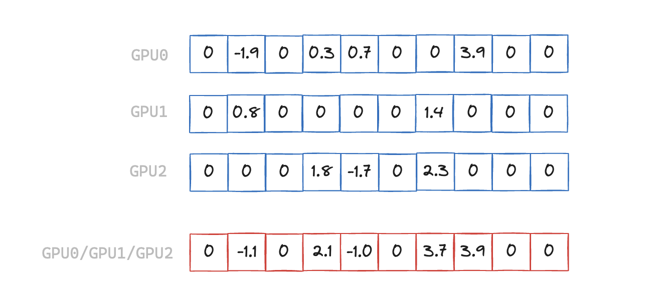 When the input arrays are sparse we can avoid transferring some elements of the array, where the result is guaranteed to be zero. In the example above we have a sparsity level of 50%, but in other real-world scenarios it can be closer to 99%.
The main steps of our sparse All-Reduce algorithm will be:
1. build_local_indices
Create a padded buffer containing the indices of the non-zero elements.
import torch
import torch.nn.functional as F

def build_local_indices(x: torch.cuda.sparse.FloatTensor) -> torch.Tensor:
    indices = x.indices()[0]
    rank = torch.distributed.get_rank()
    world_size = torch.distributed.get_world_size()
    # we need local_indices buffer to have the same size on all ranks
    # this is a requirement of NCCL's collective operations e.g. gather
    num_local_indices = indices.shape[0]
    num_local_indices_all_ranks = torch.zeros(world_size, device="cuda")
    num_local_indices_all_ranks[rank] = num_local_indices
    torch.distributed.all_reduce(num_local_indices_all_ranks)
    max_num_indices = num_local_indices_all_ranks.max().int().item()

    local_indices = F.pad(indices, (0, max_num_indices - num_local_indices), value=-1)
    return local_indices

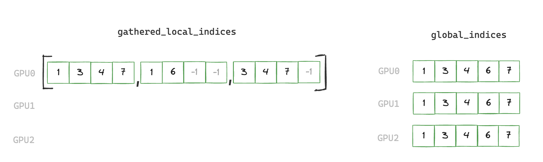
2. build_global_indices
Aggregate all local indices, then broadcast to all ranks to create global indices.
def build_global_indices(local_indices: torch.Tensor) -> torch.Tensor:
    rank = torch.distributed.get_rank()
    world_size = torch.distributed.get_world_size()
    # gather a list of tensors containing local indices from all ranks into rank 0
    gathered_local_indices = None
    if rank == 0:
        gathered_local_indices = [torch.empty(local_indices.shape[0], device="cuda", dtype=torch.int64)
                                  for _ in range(world_size)]
    torch.distributed.gather(local_indices, gather_list=gathered_local_indices)

    num_global_indices = torch.tensor(0, device="cuda")
    # de-duplicate gathered local indices on rank 0 to create global_indices
    if rank == 0:
        global_indices = torch.cat(gathered_local_indices).unique()
        global_indices = global_indices[global_indices != -1]  # remove padding
        num_global_indices.copy_(global_indices.shape[0])

    # send global_indices to all other ranks
    torch.distributed.broadcast(num_global_indices, 0)
    if rank != 0:
        global_indices = torch.empty(num_global_indices, device="cuda", dtype=torch.int64)

    torch.distributed.broadcast(global_indices, 0)
    return global_indices
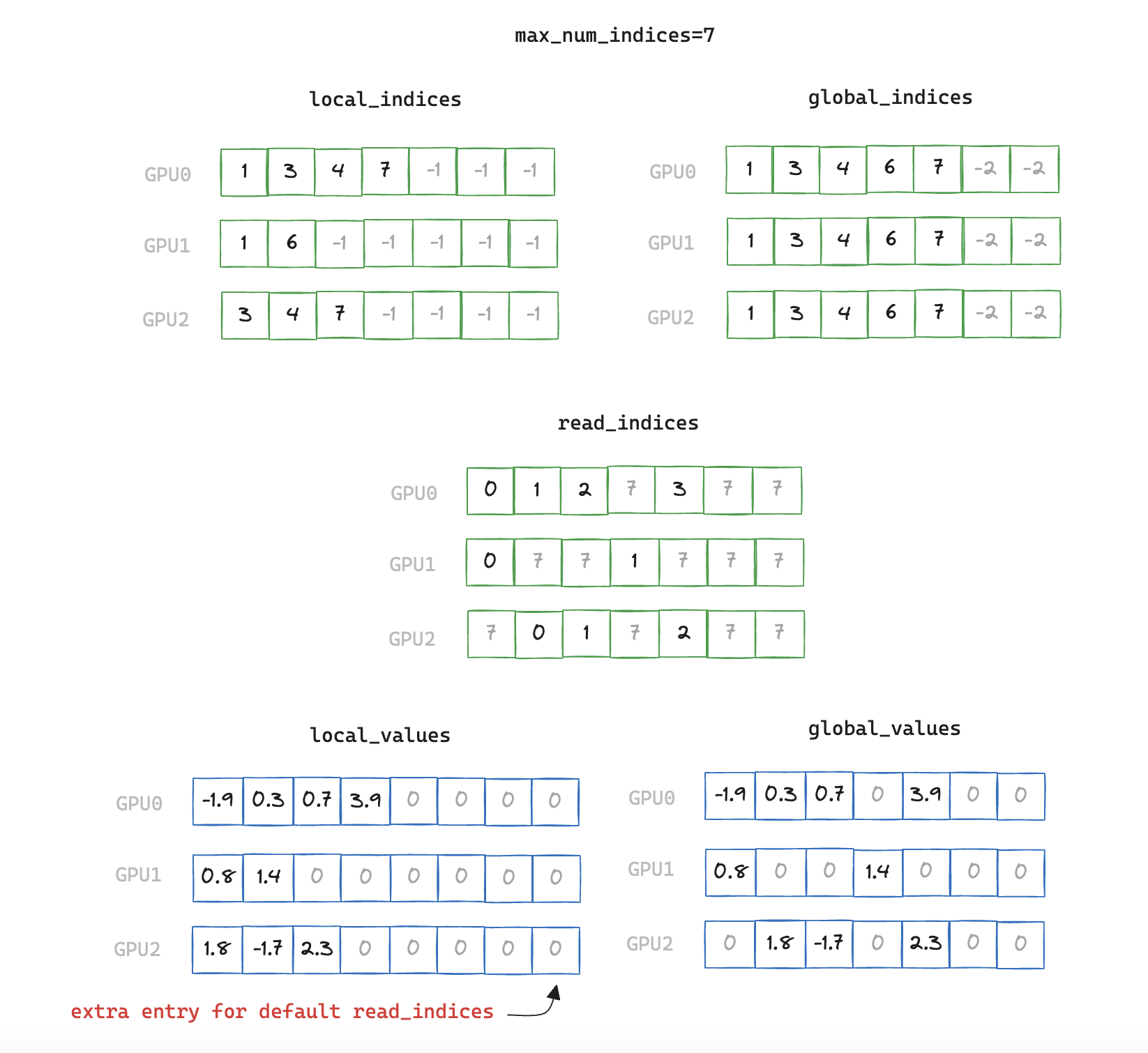
3. write_local_values_to_global_indices
We now have a de-duplicated index of all elements that are non-zero on any rank. Next we need to find the mapping between local indices and global indices, and write out the corresponding values we wish to communicate in the final All-Reduce.
Finding this mapping is necessary as the local index which matches a corresponding global index can be located at a different offset within its vector, so we have an additional stage of indirection.
def write_local_values_to_global_indices(
    x: torch.cuda.sparse.FloatTensor, global_indices: torch.Tensor
) -> torch.Tensor:
    global_values = torch.zeros(global_indices.shape[0], x.shape[1], device="cuda")

    write_indices = torch.cat([torch.nonzero(global_indices == read_index)[0]
                               for read_index in x.indices()[0]])

    global_values[write_indices] = x.values()

    return global_values
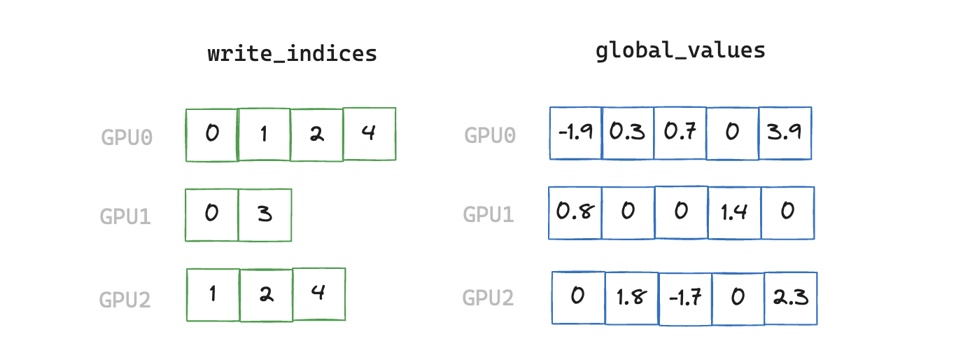
Note that we have a scalar global_value corresponding to each index in this example, but in our benchmarking runs each index will correspond to a vector of size 2048 (sourced from a sparse embedding table with 5e6 rows)
4. all_reduce
Finally we carry out the all_reduce on the target values, and convert the result to a sparse tensor.
torch.distributed.all_reduce(global_values)

output = torch.sparse_coo_tensor(global_indices.unsqueeze(0), global_values, size=x.shape, device="cuda")

v1: torch.nonzero
Putting it all together we have
def sparse_all_reduce_nccl(x: torch.cuda.sparse.FloatTensor) -> torch.cuda.sparse.FloatTensor:
    assert x.is_sparse
    assert x.dim() == 2
    x = x.coalesce() # info on this can be found in Part 1 of blog

    local_indices = build_local_indices(x)

    global_indices = build_global_indices(local_indices)

    global_values = write_local_values_to_global_indices(global_indices)

    torch.distributed.all_reduce(global_values)

    output = torch.sparse_coo_tensor(global_indices.unsqueeze(0), global_values, size=x.shape, device="cuda")

    return output
So far so good, but is it fast?

Not really 🥲
We have improved upon the Gloo sparse baseline which is good news, but it's still way off the performance of naively communicating the entire dense tensor with NCCL. Let's dig into why...
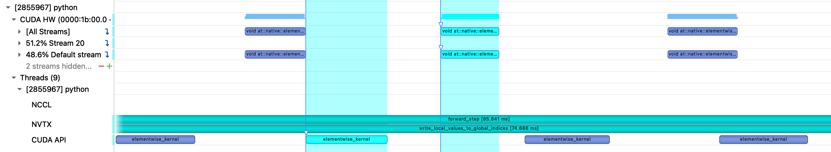
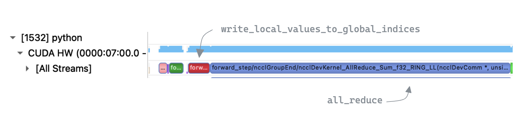
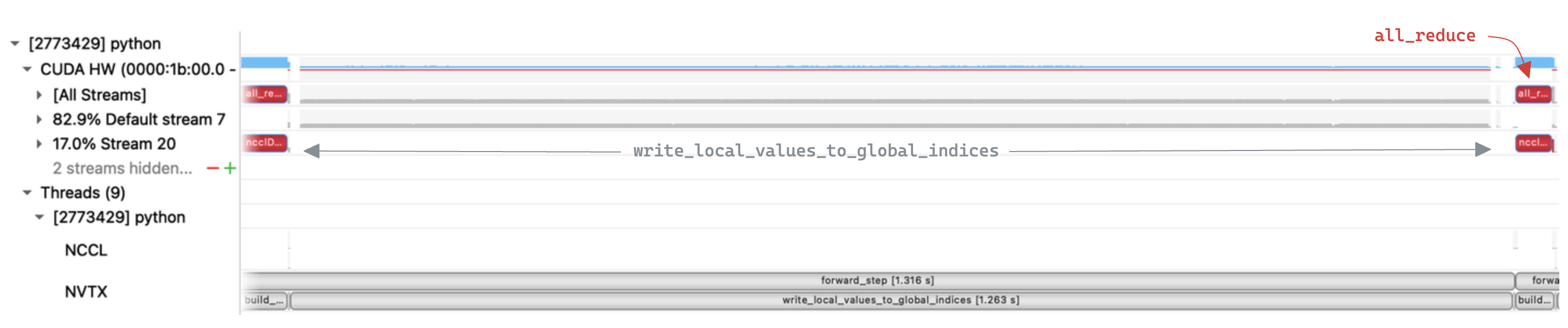 Inspecting the trace we can clearly see that
 write_local_values_to_global_indices is the bottleneck, taking up 96% of the execution time. In contrast the all_reduce step is relatively quick, suggesting there is a lot of scope for improvement in our implementation.
write_local_values_to_global_indices is dominated by a loop over local indices, to find the matching entry in global indices. Zooming in to a single iteration of that loop we see that a multiple kernels are executed, with large gaps in GPU utilization.
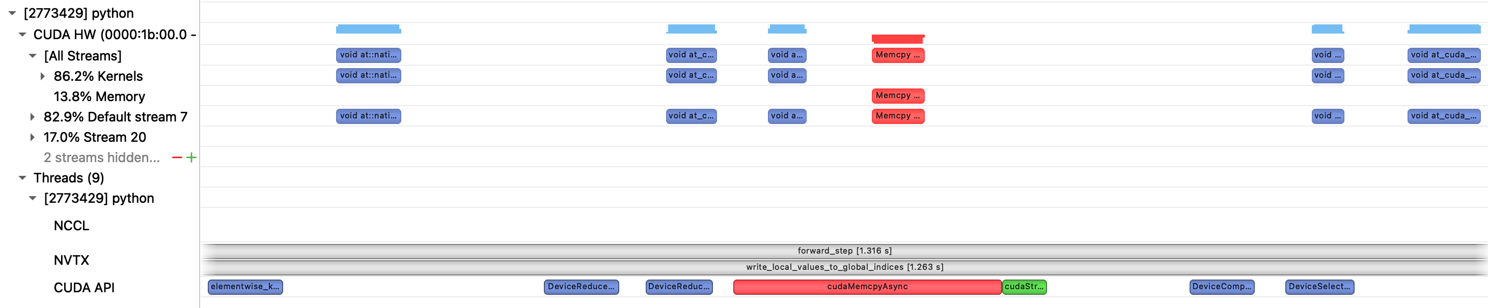
We also see an implicit synchronization point due to a device->host copy. This appears to be unavoidable as torch.nonzero need to return information to the CPU about the number of output matches, for the tensor shape metadata. This is unfortunate, as in our case we know apriori that there will be exactly one match. We now look at an alternative approach to try and avoid the synchronization.
v2: torch.where
def write_local_values_to_global_indices(
    x: torch.cuda.sparse.FloatTensor, global_indices: torch.Tensor
) -> torch.Tensor:
    global_values = torch.zeros(global_indices.shape[0], x.shape[1], device="cuda")
    local_indices = x.indices()[0]

    write_indices = torch.empty_like(local_indices, dtype=torch.int64)
    # enumerate results in host/device copy so we create counter directly on GPU
    counter = torch.arange(global_indices.shape[0], device="cuda", dtype=torch.int64)

    for step, global_index in zip(counter, global_indices):
        condition = local_indices == global_index
        torch.where(condition, step, write_indices, out=write_indices)

    global_values[write_indices] = x.values()
    return global_values
For v2 we modify write_local_values_to_global_indices to avoid using torch.nonzero. On the surface this may seem less efficient, as we are now writing out a tensor of size write_indices for every local index, rather than just once.
However in practise avoiding the synchronization point is more important, and we see improved performance!

We now have two alternating eq/where kernels per loop iteration, rather than the five kernels and a device->host copy we saw in v1. The overall duration of write_local_values_to_global_indices is now ~50% shorter. As an aside the reason that we can avoid synchronization with the host is because torch.where guarantees the shape of the output, compared to torch.nonzero which returned a size dependent on the number of matches.
However we still observe poor GPU utilization, as can be seen by the gaps between kernels. This appears to be due to the fact that each kernel is very lightweight and has a execution time (top) on the same order of magnitude as the kernel launch (bottom). This means we are never able to saturate the command queue, and the GPU is often waiting for work to be allocated to it.
A common solution for scenarios where the host-side kernel launch is the bottleneck is to use CUDA Graphs, which we will look at next.
v3: CUDA Graphs
CUDA Graphs allow us to significantly reduce the kernel launch overhead by recording a series of operations in a computational graph, then re-executing those operations on new input data. This effectively gives us a single kernel launch for the overall graph, rather than one for each kernel within it.
This sounds ideal, but there are a few caveats:
- Input/output buffer sizes must remain fixed. This is a problem for our use-case as each All-Reduce call may have a different number local / global indices.
- CUDA Graphs do not support dynamic control flow. Related to the previous point, the size of our loop is dependent on local / global which means
- CPU synchronization is prohibited. Luckily we solved this in the previous version.
To solve the issues brought about by variable number of local / global indices we can set an fixed upper bound of max_num_indices, and pad the inputs accordingly.
Obviously this is non-ideal as we cannot always know what the maximum number of indices will be for a given scenario. Also if we set the value too high we will be increasing the amount of redundant data we are sending, but this assumption will allow us to test CUDA Graphs for now.
def write_local_values_to_global_indices(
    local_values: torch.Tensor,
    local_indices: torch.Tensor,
    global_values: torch.Tensor,
    global_indices: torch.Tensor,
    max_num_indices: int,
) -> torch.Tensor:
    # default read index points to a dummy entry of zeros in local_values
    read_indices = torch.full_like(global_indices, max_num_indices, dtype=torch.int64)
    counter = torch.arange(max_num_indices, device=local_indices.device, dtype=torch.int64)

    for step, local_index in zip(counter, local_indices):
        condition = global_indices == local_index
        torch.where(condition, step, read_indices, out=read_indices)

    global_values.copy_(local_values[read_indices])
    return global_values
The general structure of the function remains unchanged, but we now write to all positions of the output tensor, compared to the previous approach of only writing selected indices. This is to ensure that all kernels in the CUDA Graph operate on fixed sizes tensors.
We also pre-allocate the input/output buffers, and pass them into the outer function as the graph always uses the same memory allocations for each execution.
def sparse_all_reduce_nccl(
    x: torch.cuda.sparse.FloatTensor,
    local_values_buffer: torch.Tensor,
    local_indices_buffer: torch.Tensor,
    global_values_buffer: torch.Tensor,
    global_indices_buffer: torch.Tensor,
    cuda_graph: torch.cuda.graphs.CUDAGraph
) -> torch.cuda.sparse.FloatTensor:

    x = x.coalesce()

    local_indices = build_local_indices(x)

    global_indices = build_global_indices(local_indices)

    # update buffers with appropriate padding
    local_indices_buffer.fill_(-1)
    local_indices_buffer[: local_indices.shape[0]] = local_indices
    local_values_buffer.fill_(0)
    local_values_buffer[: x.values().shape[0]] = x.values()
    global_indices_buffer.fill_(-2)
    global_indices_buffer[: global_indices.shape[0]] = global_indices
    # this is calling write_local_values_to_global_indices
    cuda_graph.replay()

    torch.distributed.all_reduce(global_values)

    output = torch.sparse_coo_tensor(global_indices.unsqueeze(0), global_values[:global_indices.shape[0]], size=x.shape, device="cuda")

    return output
Note that we deliberately pad local and global indices with different values. This ensures that when searching across padded values we don't achieve a "match" with both a padded local and global index. When we are unable to find a match for an index (either due to padding, or because a rank genuinely doesn't have an equivalent local value) we fall back to the default value in read_indices, which always points to values containing all zero.
Lastly we need to initialize the buffers and record the CUDA Graph itself, this is a one-off step that is executed prior to the first call to sparse_all_reduce_nccl.
def record_cuda_graph(
    x: torch.cuda.sparse.FloatTensor,
    max_num_indices: int
) -> Tuple[Tensor, Tensor, Tensor, Tensor, torch.cuda.graphs.CUDAGraph]:

    feat_dim = x.shape[1]
    indices_local_buffer = torch.empty(max_num_indices, device="cuda", dtype=torch.int64)
    indices_global_buffer = torch.empty(max_num_indices, device="cuda", dtype=torch.int64)
    values_local_buffer = torch.empty((max_num_indices + 1, feat_dim), device="cuda")
    values_global_buffer = torch.empty((max_num_indices, feat_dim), device="cuda")

    cuda_graph = torch.cuda.CUDAGraph()
    with torch.cuda.graph(cuda_graph):
        write_local_values_to_global_indices(
            values_local_buffer,
            indices_local_buffer,
            values_global_buffer,
            indices_global_buffer,
            max_num_indices
        )
    return values_local_buffer, indices_local_buffer, values_global_buffer, indices_global_buffer, cuda_graph
Note the additional position we create for values_local_buffer, this is to guarantee that we write zeros when no match between indices is found.
After running our benchmark we see performance has improved again 🥳

We can now see a (single) CUDA Graph launch in the trace when looking at a call to sparse_all_reduce_nccl, as expected.
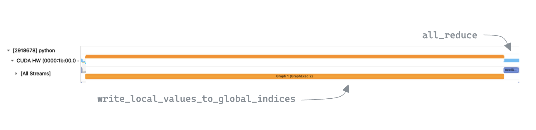 One interesting thing to note is that despite
 write_local_values_to_global_indices now running faster, its % contribution to the overall execution time is similar to v1. This is because the time taken by the all_reduce is now shorter on average, which is surprising as the amount of data it is communicating has not changed.
In reality this is because v1 had more interactions with the CPU via many kernel launches / synchronization points, resulting in more variance in timings for write_local_values_to_global_indices.
This meant that GPUs which were first to reach all_reduce would have to wait for the slowest GPU to catch up before being able to actually execute the collective. This "waiting for stragglers" is captured within the kernel execution time, so all_reduce is technically not quicker, but is still a nice side-effect of making the loop runtime more consistent in the distributed setting.
We can also inspect the recorded CUDA Graph with cuda_graph.enable_debug_mode:

This illustrates the "for loop" unrolled into the fixed number of iterations which were encountered when the CUDA Graph was recorded. Here we show only 6 iterations (alternating between calls to where and eq kernels), but the graphs in our benchmark have ~50,000.
With CUDA graphs we are now approaching the performance of the dense NCCL baseline, but we still aren't seeing any benefits from sparsity. In addition to this, the extra complexity and padding does not provide a particularly enticing trade-off, but we can potentially simplify things with a recent addition to PyTorch: CUDA Graph Trees 🌲.
CUDA Graph Trees should allow us to remove the max_num_indices constraint and the need for manual padding, as it provides support for dynamic input sizes. It works by creating a single buffer for each input/output/intermediate, and then each graph invocation (corresponding to a specific shape) is simply a pointer offset into that allocation. However this would mean recording graphs on the fly as new input shapes were encountered (slow), and despite notionally supporting branching logic, its ability to handle the variable length loop would need to be tested
In any case it seems that our sparse All-Reduce is still dominated by write_local_values_to_global_indices. One improvement we could make is to forgo the loop entirely and parallelize the index search on the GPU, which we will look at next.
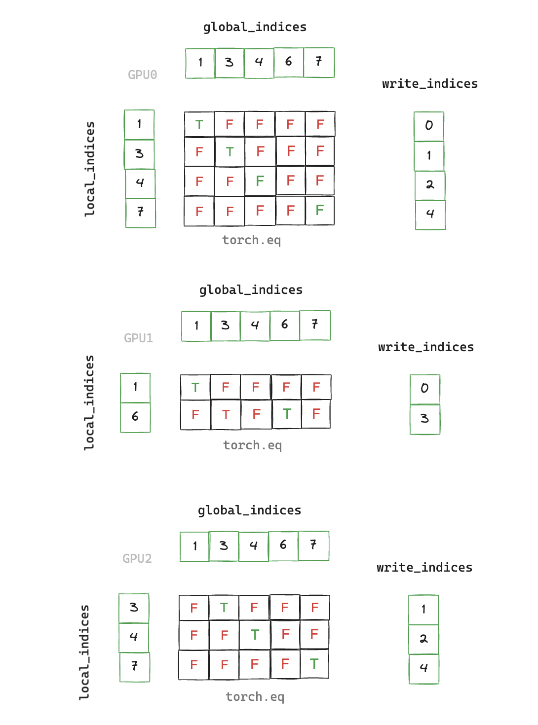
v4: broadcast torch.eq
write_local_values_to_global_indices requires us to take each local index and find the corresponding position of the matching global index. This problem is embarrassingly parallel and if we assume that each iteration of our loop is not fully utilizing the GPU SMs, it seems reasonable that parallelizing the search could lead to performance gains.
Furthermore, the current loop will be loading the target indices from DRAM -> SRAM on every iteration. Fusing these loads into a single kernel should help improve what is very likely a memory-bandwidth bound scenario.
Can we parallelize the search using PyTorch native operations? We currently call torch.eq implicitly on each loop iteration when creating the condition used by torch.where / torch.nonzero e.g.
for step, global_index in zip(counter, global_indices):
    condition = local_indices == global_index
    # equivalent to torch.eq(local_indices, global_index)
    torch.where(condition, step, write_indices, out=write_indices)
The torch.eq docs tells us that the second argument is broadcast-able. So rather than doing a vector/scalar operation as before, by satisfying the conditions for broadcasting semantics we can carry out a vector/vector operation over the entire indices tensors:
def write_local_values_to_global_indices(
    x: torch.cuda.sparse.FloatTensor,
    global_indices: torch.Tensor,
) -> torch.Tensor:

    local_indices = x.indices()[0]
    global_values = torch.zeros(global_indices.shape[0], x.shape[1], device="cuda")
    # max() returns index of max value as second return value
    # equivalent to argmax, which is unsupported for bool type tensors
    write_indices = torch.eq(local_indices.unsqueeze(0),
                             global_indices.unsqueeze(1)).max(dim=0)[1]

    global_values[write_indices] = x.values()

    return global_values

Now we're cooking with gas! 🚀 We finally have all sparse All-Reduce that is faster than it's dense counterpart, and by some distance! However its not all good news...
As we carry out the argmax reduction as a separate operation, we have to materialize the entire boolean output from torch.eq into DRAM. Not only will this write/read potentially be expensive, it also means a large memory footprint. For the local indices we are using for benchmarking (size ~50k) this translates to a 9.3GB tensor 😕.
What we really want is a single fused kernel that carries out both the eq and argmax before writing the fully reduced output.
v5: CUDA kernel
We implement a CUDA kernel to carry out the local -> global index matching operation
__global__ void invert_index_kernel(
  const int* local_indices, const int* global_indices, int* output_indices,
  int local_indices_size, int global_indices_size
) {
  extern __shared__ int smem[];

  // load local_indices
  int local_index = -1;
  int local_index_offset = blockDim.x * blockIdx.x + threadIdx.x;
  if (local_index_offset < local_indices_size) {
    local_index = local_indices[local_index_offset];
  }

  int global_index_tiles = ceil(global_indices_size / static_cast<float>(blockDim.x));

  for (int i = 0; i < global_index_tiles; i++) {
    __syncthreads(); // ensure threads have finished previous search before loading next tile into shared memory
    // load global_indices
    int global_index_offset = i * blockDim.x + threadIdx.x;
    if (global_index_offset < global_indices_size) {
      smem[threadIdx.x] = global_indices[global_index_offset]; // avoid out of bounds read
    }
    __syncthreads();

    // iterate over global_indices in current tile searching for match
    for (int j = 0; j < blockDim.x; j++) {
      if (i * blockDim.x + j >= global_indices_size) {
        break;
      }
      if (smem[j] == local_index) {
        output_indices[local_index_offset] = i * blockDim.x + j;
        break;
      }
    }
  }
}
Apply appropriate Python bindings to launch the kernel
#include "cuda_runtime.h"
#include <iostream>
#include <stdio.h>
#include <torch/extension.h>

torch::Tensor invert_index_v1(torch::Tensor local_indices, torch::Tensor global_indices) {
  auto output = torch::empty_like(local_indices, torch::TensorOptions().dtype(torch::kInt));
  int threads_per_block = 256;
  int blocks = ceil(local_indices.size(0) / static_cast<float>(threads_per_block));
  int shared_memory_size = (threads_per_block) * sizeof(int);

  invert_index_kernel_v1<<<blocks, threads_per_block, shared_memory_size>>>(local_indices.toType(torch::kInt).data_ptr<int>(),
                                                                         global_indices.toType(torch::kInt).data_ptr<int>(),
                                                                         output.data_ptr<int>(), local_indices.size(0), global_indices.size(0));
  AT_CUDA_CHECK(cudaGetLastError());
  AT_CUDA_CHECK(cudaDeviceSynchronize());
  return output;
}

PYBIND11_MODULE(TORCH_EXTENSION_NAME, m) {
  m.def("invert_index", &invert_index, "match local indices to global indices");
}
And lastly update write_local_values_to_global_indices
def write_local_values_to_global_indices(
    x: torch.Tensor,
    global_indices: torch.Tensor,
) -> torch.Tensor:
    local_indices = x.indices()[0]
    global_values = torch.zeros(global_indices.shape[0], x.shape[1], device="cuda")
    write_indices = sparse_all_reduce.invert_index(local_indices, global_indices)

    global_values[write_indices] = x.values()

    return global_values
After tuning the block size and benchmarking we see our performance is ahead of v4. Not only this, but we have also achieved our goal of the avoiding the O(N²) memory requirements of torch.eq as the search is carried out in a single fused kernel.

What is perhaps most surprising it that we see good performance from this relatively naive kernel, as it only uses a fraction of the GPU's available streaming multiprocessors. This low occupancy is due the fact that our problem size of ~50k indices is relatively small. Each thread is responsible for processing a single local index, but the H100 is capable of having ~300k threads resident concurrently.
Next we look at optimizing the CUDA kernel to better utilize the GPU.
v6: CUDA (optimized)
The main shortcoming of v5 was that the GPU's compute capacity was left under-utilized. We can fix this by re-distributing our workload and assigning more than one thread to each local index.
__global__ void invert_index_kernel(
  const int* local_indices, const int* global_indices, int* output_indices,
  int local_indices_size, int global_indices_size, int local_indices_per_block
) {
  extern __shared__ int smem[];

  int global_index_tiles = ceil(global_indices_size / static_cast<float>(blockDim.x));

  // load local indices into shared memory
  int local_index_offset = local_indices_per_block * blockIdx.x + threadIdx.x;
  if ((local_index_offset < local_indices_size) && (threadIdx.x < local_indices_per_block)) {
    smem[threadIdx.x] = local_indices[local_index_offset]; // avoid out of bounds read
  } else if (threadIdx.x == local_indices_per_block) {
    smem[threadIdx.x] = 0; // reset thread block level match counter
  }
  __syncthreads();

  int global_index;
  // start iteration from first tile that could potentially contain a match
  int global_index_tile = local_indices_per_block * blockIdx.x / blockDim.x;
  for (global_index_tile; global_index_tile < global_index_tiles; global_index_tile++) {
    int global_index_offset = global_index_tile * blockDim.x + threadIdx.x;
    if (global_index_offset >= global_indices_size) {
      return;
    }
    // exit early if all local_indices have found a match
    if (smem[local_indices_per_block] == local_indices_per_block) {
      return;
    }
    // load globals indices for each tile into local registers
    global_index = global_indices[global_index_offset];

    for (int smem_local_index_offset = 0; smem_local_index_offset < local_indices_per_block; smem_local_index_offset++) {
      local_index_offset = local_indices_per_block * blockIdx.x + smem_local_index_offset;
      if (local_index_offset >= local_indices_size) {
        break;
      }
      int local_index = smem[smem_local_index_offset];

      if (global_index == local_index) {
        output_indices[local_index_offset] = global_index_offset;
        atomicAdd(&smem[local_indices_per_block], 1); // avoid race conditions between threads
      }
    }
  }
}
Specifically all the threads in a single thread block now execute the search in parallel for a given local index. This increases the degree of parallelism by blockDim.x and means we are now able to oversubscribe the SMs on the GPU for the same problem size, achieving much higher occupancy.
We illustrate this in the following toy example, for a small number of threads/blocks, where the x-axis represents global_indices and the y-axis represents local_indices.
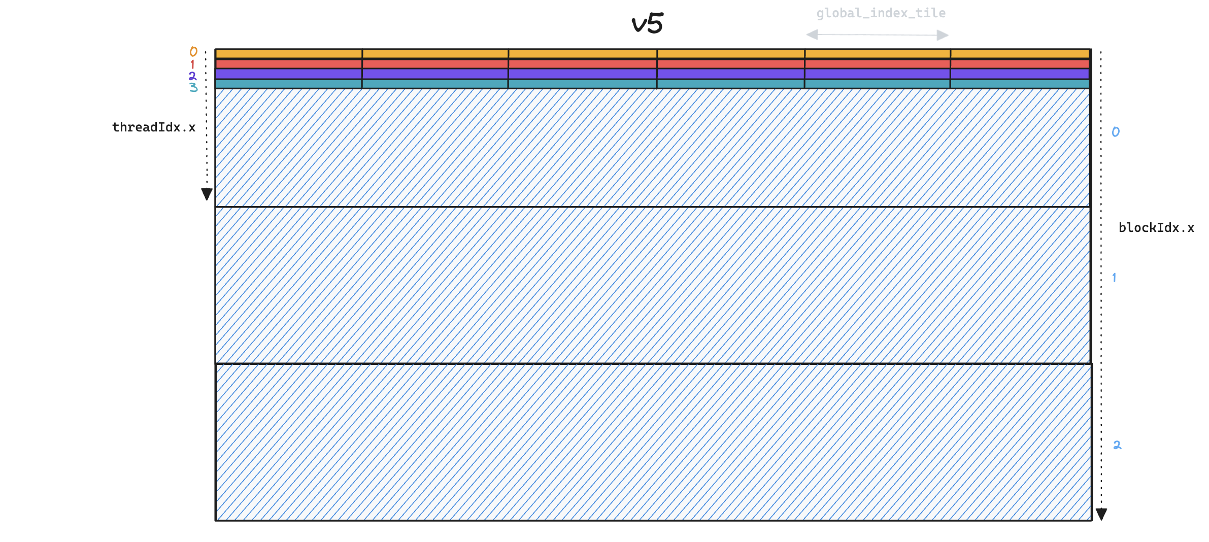 Whilst each thread in v5 (above) iterates over all
 global_indices, in v6 (below) each thread only processes a single global_index per global_index_tile, and so we end up launching many more thread blocks.
 Memory access patterns have also changed, in v5 we read
 global_indices into shared memory, requiring only a single SRAM load per global index for each thread block. In v6 this pattern is no longer necessary as threads are now responsible for processing distinct global indices, so we can simply use local registers.
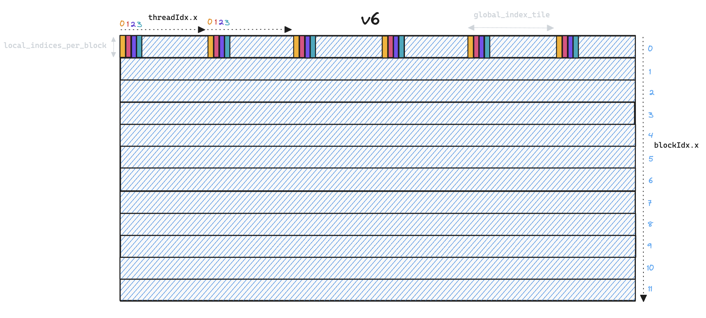
However, we are faced with a performance trade-off as increased parallelism means we have to load each global index once per local index, instead of sharing them across all local indices in a thread block. We solve this by processing multiple local_indices in each thread block, essentially transposing the problem from v5 where a single thread iterated over multiple global_indices, to v6 where a single thread iterates over multiple local_indices.
The choice of local_indices_per_block is important. At one extreme we process a single local index per block for maximum parallelism, but are memory-bandwidth bound as we maximize the number of DRAM->SRAM reads of global_indices. At the other extreme a large value of local_indices_per_block will amortize the cost of loading global_indices, but also means more serial work for each thread, which will approach the performance of v5 in the limit.
In practise we want local_indices_per_block to sit somewhere in the middle, which we can see illustrated below:
- ID 0:
local_indices_per_block=1 - ID 1:
local_indices_per_block=8 - ID 2:
local_indices_per_block=64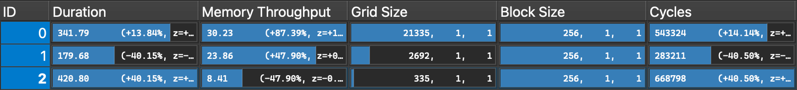 As expected, when processing 64 local indices per block we see lower memory throughput as we require fewer
 global_indicesreads from DRAM. However this also means a low degree of parallelism as we only launch 335 blocks, which results in higher execution time. Reducinglocal_indices_per_blockimproves performance, but only up to a point beyond which excessive loading of global_indices becomes the bottleneck.
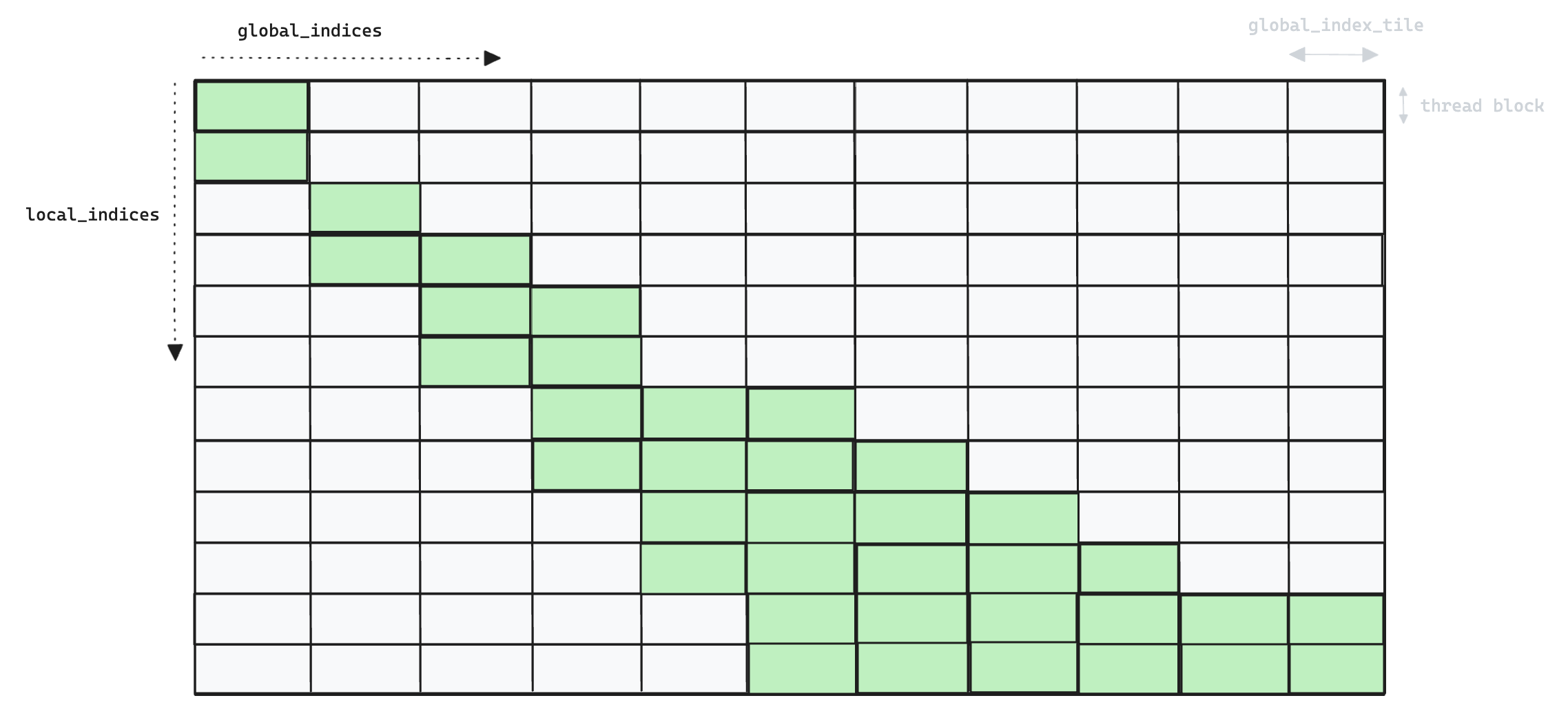
The second significant optimization in v6 is the reduction of redundant computation. In v5 we naively check every local_index against every global_index, but in v6 we compute global_index tiles in a more selective manner.
- We track which local indices have found a match, and short-circuit the
global_index_tileloop after all local indices in the current thread block have been matched. - We exploit the fact that local_indices and global_indices are ordered, and local_indices and a subset of global_indices. This allows us to calculate the offset of the minimum
global_index_tilewhich could potentially contain a match.
The following image shows an example pattern of the global_index tiles that actually get computed in v6.
 A more granular approach that skipped "already matched" local indices in the inner-loop was also tested. However, in practise the check for completed indices was found to be just as expensive as the check for
 local_index == global_index, with both using the same ISETP.NE.AND PTX instruction for integer comparison.
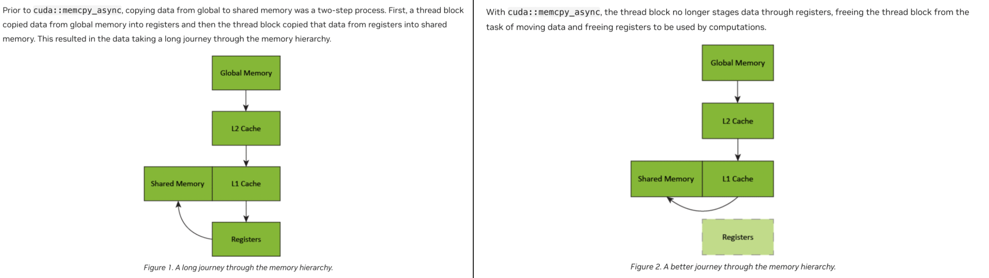
Lastly we look into minimizing the cost of loading global indices from DRAM->SRAM by using the cuda::memcpy_async API first introduced in the Ampere generation (not to be confused with cudaMemcpyAsync, which is responsible for host<->device copies).
We create a multi-stage pipeline with a rotating buffer in shared memory, to ensure that the global_indices for tile N+1 are being loaded whilst tile N is being processed. Note that the pipeline scope is at the thread level, as we do not require co-operation between all threads in the block as previous mentioned.
extern __shared__ int smem[];
constexpr size_t stages_count = 2;
int smem_offset[stages_count] = {local_indices_per_block + 1, local_indices_per_block + 1 + blockDim.x};
cuda::pipeline<cuda::thread_scope_thread> pipeline = cuda::make_pipeline();
int compute_tile = 0;
int fetch_tile = 0;
We also replace global_index = global_indices[global_index_offset]; with the following inner loop, which is responsible for orchestrating the loading of data into shared memory. The first time the loop is entered we load two global indices asynchronously (to fill the buffer) then on each successive global_index_tile we pre-fetch a single item.
while (fetch_tile < global_index_tiles && fetch_tile < (compute_tile + stages_count)) {
    pipeline.producer_acquire();
    int smem_idx = fetch_tile % stages_count;
    int global_offset = (global_index_tile + smem_idx) * blockDim.x;
    cuda::memcpy_async(smem + smem_offset[smem_idx], global_indices + global_offset, sizeof(int) * blockDim.x, pipeline);
    pipeline.producer_commit();
    fetch_tile++;
}

pipeline.consumer_wait();
__syncwarp()
int smem_idx = compute_tile % stages_count;
global_index = smem[smem_offset[smem_idx] + threadIdx.x];
compute_tile++;
Note that whilst we do not need co-operation across the whole thread block, we still synchronize at the warp level to avoid potential warp divergence.
It is also worth noting that we actually have no need to use shared memory as each thread is responsible for loading it's own global index directly into a local register. This pattern is simply to satisfy the memcpy_async API. Typically loading into shared memory means the data is staged via a register on its way to shared memory, which is suboptimal. An additional benefit memcpy_async provides is to avoid this additional hop, which is good news, but for our use-case we would ideally avoid shared memory altogether
When measuring the updated performance we see that unfortunately the addition of cuda::memcpy_async does not surpass our v6 performance with the existing optimizations. This could be due to additional operations associated with the pipeline (e.g. offset calculations) as the "computation" in our kernel is very lightweight, so any extra overhead will be disproportionately expensive.
It could also be due to the fact that we can already hide latency of loading data into SRAM by oversubscribing the warp scheduler. The main benefit of cuda::memcpy_async is to remove the requirement of other (eligible) warps to hide the latency i.e. data movement can now be pipelined within the context of a single warp.
Lastly, the lack of async gains may be because the relatively small size of the indices vectors means that most of the data persists resident in the L1 cache, and profiling reveals we have an L1 cache hit-rate of 84.6% for global memory loads.
To recap the v6 optimizations which did make the final-cut are:
- Transpose the problem to parallelize across
global_indicesand increase the number of thread blocks - Exploit ordering of indices vector to offset the start of the search and reduce the number of tiles we need to search over
- Exit early when all matches have been found for a single thread block
The combination of all v6 optimizations results in an 12x speedup over v5 for the invert_index kernel, and this translates to the following overall improvement in the sparse All-Reduce.

Despite the large kernel speed-up, the smaller end-to-end improvement shows that we have now reached a point where write_local_values_to_global_indices is no longer a significant bottleneck.
Next steps
We have achieved our goal of exploiting the reduced data communication required for a sparse All-Reduce and observe significant performance gains 🚀
Some possible future directions:
- Look into using TensorIterators to avoid requiring a custom CUDA kernel for a performant index lookup.
- Currently our new
all_reduceis run standalone after the backwards pass. Ideally we would overlap its execution with the backwards, potentially using PyTorch communication hooks. - The latest version of PyTorch hints at future support for an experimental sparse All-Reduce in NCCL. It would be interesting to benchmark and compare implementations when it becomes available.
- PyTorch will perform the device-host copy for us, but doing it explicitly is convenient as it allows us to measure the cost of the copy, and benchmark NCCL and Gloo based collectives in the same distributed context (by setting
backend=None)↩