Reduce Model Tuning Costs with MuP

As machine learning engineers increasingly adopt the Bitter Lesson and models grow in size, the cost associated with training them is also on the rise. A significant portion of overall compute budget is frequently spent on hyper-parameter tuning before launching a final training run. MuP offers the capability to transfer hyperparameters from a much smaller 'toy' model, leading to a substantial reduction in overall training cost.

Typically the optimum hyperparameter setup for small and large models, even with the same architecture, differs significantly. This means that hyperparameter tuning needs to be conducted on full sized models. We typically run the sweep for a small number of steps, then extrapolate, introducing a degree of uncertainty.

MuP (Maximal Update Parametrization) re-parametrises a model in such a way that most hyper-parameters are directly transferable across model sizes. This allows you to tune on small models for the full number of steps, then directly transfer those hyper-parameters across to a larger model for the final training run.

How Does MuP Work?

Intuition

Here we outline an intuition behind why MuP works. For a full proof refer to the original paper.

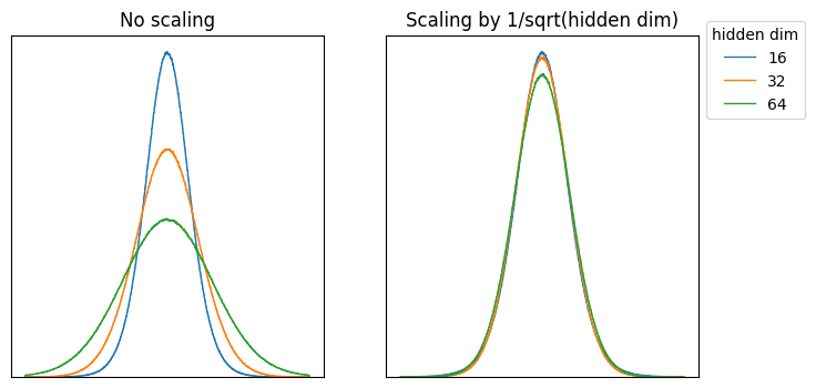
The key intuition behind MuP is that activations need to be kept within a constant dynamic range across model scales in order for optimal hyperparameters to remain constant across those scales. What we want to avoid is the situation on the left, where the output distribution varies according to the dimensions of the model. Instead, we would like the output distribution to be invariant, as shown on the right.

A linear layer can be thought of as a series of dot products performed in parallel. As we scale the hidden dimension of the model, the vectors that are used to calculate each dot product get larger. For input values (and model weights) drawn from a standard normal distribution, the standard deviation of the output distribution will grow with the size of the hidden dimension (left hand plot below).

However, if we scale the model weights by $\frac{1}{\sqrt{d_{in}}}$ we see that the output distribution remains virtually the same across different input dimensions (right hand plot). This is the essence of what MuP is trying to achieve through initialisation.

However, as training proceeds, the weight matrix is altered through gradient updates. We therefore need to ensure that the invariance described above holds throughout training and not just at initialisation. To simplify this problem it helps to reformulate the forward pass. Take a parameter ($W$) which has had a single gradient update applied ($\Delta{}W$). We would usually model the subsequent forward pass as follows:

$$z = (W + \Delta{}W)x$$

However, due to the linearity of the update, we can instead divide it into two parallel processes: a forward pass involving the original parameter and a separate forward pass involving the gradient update. These results are then added together to give the final output:

$$z = Wx + \Delta{}Wx$$

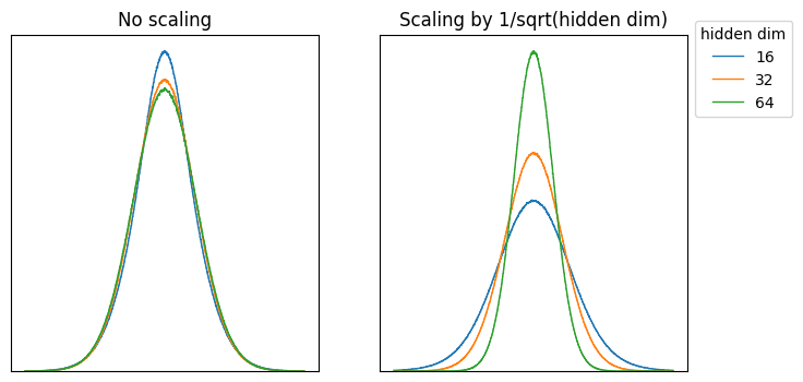
The distribution of $Wx$ has already been considered above and is only dependent on initialisation. We are therefore interested in the distribution of $\Delta{}Wx$ and how it scales with model size. During backpropagation, $\Delta{}W$ is calculated as the tensor product of $x$ and $\frac{dL}{dz}$. We can therefore reformulate $z = \Delta{}Wx$ as:

$$z_t = x_{t-1}^T\frac{dL}{dz_{t-1}}x_t$$

Each of these three vectors can be modelled as IID and we can see on the left below that, if we scale the model dimension without introducing any additional factors, the output distribution is unchanged. We therefore do not need to scale the learning rate according to model dimension and should keep it the same. If we contrast this and scale the learning rate with the inverse square root of model width ($1/\sqrt{n}$) (right hand plot) we see the same behaviour is not observed:

Which Hyper-Parameters Can Be Transferred?

The main limitation of MuP concerns regularisation. MuP works best in an infinite-data regime. Hyper-parameters that are related to regularisation, such as weight decay, do not transfer.

Nearly all other hyper-parameters have been shown empirically to transfer well using MuP:

Results

We report results here for scaling learning rate across model width (hidden dimension) and the number of layers. The model used for these experiments is a standard encoder-only transformer architecture with only minor differences from that described in the original transformer paper. We observe that the optimum learning rate remains constant at 0.0005 when scaling across both dimensions.

Implementing MuP

Setting Up MuP

Here we discuss implementing MuP for Transformer-based models. The one architectural modification that needs to be taken into account when moving over to using MuP is to scale the attention scores by $\frac{1}{d}$ rather than $\frac{1}{\sqrt{d_{in}}}$.

The only other changes concern how to scale the initial variance and per-layer learning rates of the model when moving between model sizes.

1. Initial variance: The initial variance of the elements in each parameter should scale with $\frac{1}{d_{in}}$, where $d_{in}$ is the input dimension of that parameter weight. PyTorch scales like this by default anyway. The only difference is the final output layer which projects from the hidden dim of the model to the output embedding, usually the vocabulary size: this should scale with $\frac{1}{d_{in}^2}$
2. Learning rates: Assuming you're using an Adam-based optimizer, the learning rate of each layer should scale with $\frac{1}{d_{in}}$ as the model increases in size, except for input layer mapping from the input dim to the hidden dim which should stay constant.

The MuP Package

Microsoft provide their own package, available via pip, to manage the parametrization of your model and ensure it conforms with MuP. We provide a walkthrough here for a Transformer-based model with an Adam-based optimizer. Implementations may vary slightly for other setups so refer to the original paper.

1. Alter the denominator in the attention calculation to scale with $\frac{1}{d}$ rather than $\frac{1}{\sqrt{d}}$. The authors suggest two possible approaches:

# baseline
attention = query @ key.T * 1 / math.sqrt(d)

# a) apply a fixed constant (λ) so that the 
# resulting attention scores are not too small 
attention = query @ key.T * λ / math.sqrt(d)

# b) use a fixed denominator (e.g. 32) 
# (they encountered a noisy hyper-parameter 
# landscape when d became too small)
attention = query @ key.T * 1 / λ

2. Set base shapes to obtain scaling factors

from mup import set_base_shapes

# Near the top of your training script:
base_model = # instantiate the smaller model you will run hyperparameter sweeps on
model = # instantiate the full sized model you wish to train
model = set_base_shapes(model, base_model)

set_base_shapes() calculates a 'width multiplier' for each parameter by calculating the ratio $d_{model}/d_{model\_base}$, where $d_{model}$ and $d_{model\_base}$ are the width of the respective layers. This is then accessed by MuAdam and MuReadout to scale the initial variance and per-layer learning rate appropriately. This step must therefore occur before instantiating the optimiser.

3. Use MuAdam instead of Adam

from mup import MuAdam

optimizer = MuAdam(model.parameters(), impl=torch.optim.Adam, **optimizer_kwargs)

The MuAdam wrapper divides the model parameters into separate param groups and assigns each group its own learning rate, scaled by the width multipliers calculated by set_base_shapes(). Note the MuP package only supports SGD, Adam and AdamW.

4. Replace nn.Linear with MuReadout for the unembedding layer

from mup import MuReadout

class MyModel(nn.Module):
    def __init__(self, ...):
        ...
        self.unembed = MuReadout(hidden_dim, output_dim)
        ...

MuReadout is a wrapper around nn.Linear and scales the initial variance of the weight using the width multiplier calculated by set_base_shapes(). The input to the output layer is multiplied by a scalar, output_mult, which should be swept in order to find an optimum value. This scalar is scaled by the width multiplier and so can be transferred across model sizes and only needs to be tuned once.

Implementing MuP Yourself

The MuP package only supports SGD, Adam-based optimizers out of the box. Given this, and the relative simplicity of MuP, we opted to implement MuP ourselves. This can be done in ~80 lines of code and our implementation, which can be found here, is compatible with any PyTorch optimizer.